Chapter 4 Centrality measures
Centrality measures can help us understand the internal dynamics of the network. There are several centrality measures. In this case, we will focus on the following ones:
- Degree centrality: It measures the number of connections of a node. It is the number of edges that a node has. It is a measure of the importance of a node in the network. The more connections a node has, the more important it is.
- Betweenness centrality: It measures the number of shortest paths that pass through a node. It is a measure of the influence of a node in the network. The more shortest paths pass through a node, the more influence it has.
- Closeness centrality: It measures the average distance between a node and all other nodes. It is a measure of the centrality of a node. The closer a node is to all other nodes, the more central it is.
4.1 Degree
We can start by checking the degree of each node. which simply counts the number of relationships each actors has with the other members of the sample.
In other terms, the degree of a node is the number of edges connected to the node. In terms of the adjacency matrix \(A\), the degree for a node indexed by \(i\) in a network is
\[ k_i=\sum_j a_{ij}, \]
where \(a_{ij}\) is the adjacency matrix of the network.
In our case, since the network is directed, we will focus on the in-degree and out-degree. The in-degree of a node is the number of edges that point to the node.
In terms of the adjacency matrix \(A\), the in-degree for a node indexed by \(i\) in a network is
\[ k_i^{\text{in}}=\sum_j a_{ij}, \]
Conversely, in terms of the adjacency matrix \(A\), the out-degree for a node indexed by \(i\) in a network is
\[ k_i^{\text{out}}=\sum_j a_{ji}, \]
In our context, a node that has a high in-degree means that an account is followed by many other accounts. Having a high out-degree means that an account follows many other accounts.
# Compute in and out degree
nodes$indegree <- degree(network, mode = "in")
nodes$outdegree <- degree(network, mode = "out")
We can check the summary statistics of the in-degree.
summary(nodes$indegree)## Min. 1st Qu. Median Mean 3rd Qu. Max.
## 0.0 109.5 139.0 133.4 163.5 350.0The nodes with the highest in-degree are:
## [1] "debbie stabenow" "lisa murkowski"  "doug jones"      "katie porter"
## [5] "joe courtney"    "kyrsten sinema"
We can now visually represent the in-degree using a boxplot.
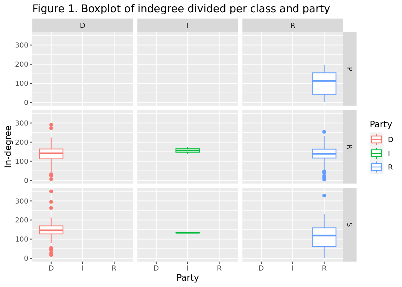
In the case of the indegree (Figure 1), the distribution is more similar across the three classes. However, the Republicans tend to have a higher indegree than the Democrats in the House of Representatives. In the Senate, the distribution is more similar. In the cabinet, the distribution is highly skewed, with some individuals having a very high indegree, while others have a very low indegree, similarly to the outdegree.
Additionally, some individuals in the House of representatives and in the cabinet have a very high indegree, this is justifiable because they are very well known as they occupy high positions in the government and therefore a higher number of officials are interested in following their tweets.
We can also visually check whether the indegree is normally distributed or not.
## `stat_bin()` using `bins = 30`. Pick better value with `binwidth`.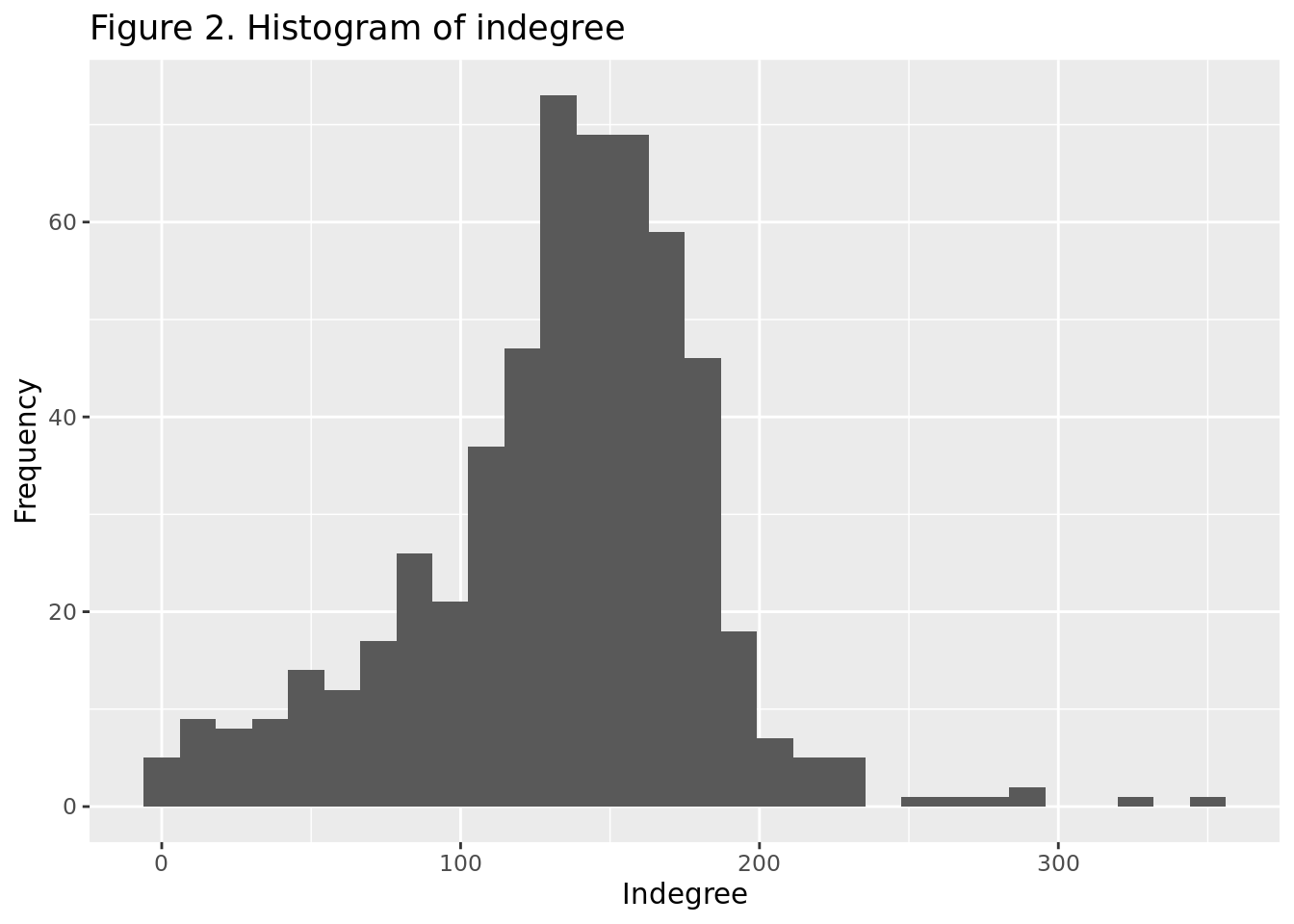
As we can see in Figure 2, the indegree is not normally distributed. This was expected, as we can see in Figure 2 that the distribution is highly skewed towards the left because of the presence of some accounts with a very high indegree and some accounts with an indegree of zero.
We can also check the summary statistics of the out-degree.
summary(nodes$outdegree)## Min. 1st Qu. Median Mean 3rd Qu. Max.
## 0.0 64.0 117.0 133.4 191.0 523.0The nodes with the highest out-degree are:
## [1] "billy long"   "mike johnson" "john rose"    "trent kelly"  "dina titus"
## [6] "tom reed"
We can now visually represent the out-degree using a boxplot.
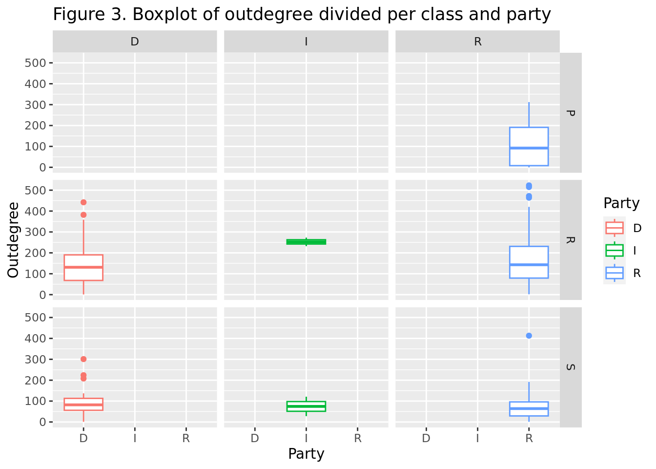
As we can see in Figure 3, the Republicans tend to have a higher outdegree than the Democrats in the House of Representatives. However, the Democrats tend to have a higher outdegree than the Republicans in the Senate. In the cabinet, the distribution is highly skewed, with some individuals having a very high outdegree, while others have a very low outdegree, if not zero. This suggests that some individuals are very active in the network, while others are not.
We can also visually check whether the outdegree is normally distributed or not.
## `stat_bin()` using `bins = 30`. Pick better value with `binwidth`.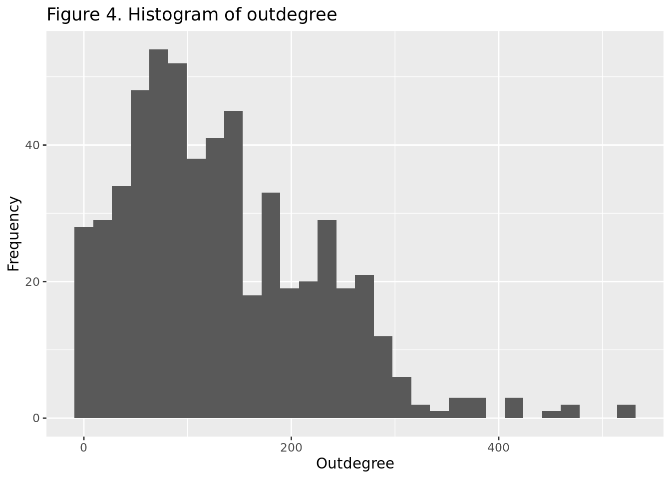
As we can see in Figure 4, the outdegree is not normally distributed.
The p-value is way below 0.05, which means that we can reject the null hypothesis and conclude that the outdegree is not normally distributed. This was expected, as we can see in Figure 2 that the distribution is highly skewed towards the left because of the presence of some accounts with a very high outdegree and some accounts with an out degree of zero.
4.1.1 Is there a relationship between the out-degree and the in-degree?
We now want to check if there is a linear relationship between the indegree and the outdegree. We can do this by running a linear regression. The indegree will be the dependent variable and the outdegree will be the independent variable.
First, we need to remove group-specific outliers, as they can affect the results of the regression. We will remove the data points that are more than 2 standard deviations away from the mean. Additionally, we will remove the data points that belong to the independents and the cabinet, as there is not enough data to perform a regression.
Now we can run the regression.
## `geom_smooth()` using method = 'loess' and formula = 'y ~ x'
As we can see in Figure 5, there seem to be a sort of positive relationship between the indegree and the outdegree. However, the relationship is not very strong, as there is high variability in the data points.
We can check the distribution of the residuals using a histogram and perform a Shapiro-Wilk test to check if the residuals are normally distributed.
## `stat_bin()` using `bins = 30`. Pick better value with `binwidth`.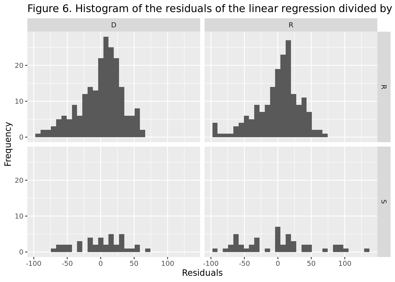
## `summarise()` has grouped output by 'class'. You can override using the
## `.groups` argument.| class | party | p.value |
|---|---|---|
| R | D | 0.0000824 |
| R | R | 0.0000509 |
| S | D | 0.3042314 |
| S | R | 0.1049630 |
The p-value for the House of Representatives is way below 0.05, which means that we can reject the null hypothesis and conclude that the residuals are not normally distributed. The p-value for the Senate is higher than 0.05, which means that the residuals are normally distributed. However, we cannot jump to the conclusion that there is a linear relationship between the indegree and the outdegree, as there are many other social factors that can may affect the results of the regression. For example, the usage rate of the Twitter account, the digital literacy of the individual, whether it is an account managed by the politician or by an external team, etc.
4.2 Betweenness Centrality
The betweenness centrality measures the extent to which a vertex lies on paths between other vertices. Vertices with high betweenness may have considerable influence within a network by virtue of their control over information passing between others. They are generally characterized by a high in-degree and can start viral content which can be reposted by other members of the network.
In this case, whether the network is directed or undirected is relevant, as the flow of information is monodirectional. The betweenness centrality of a node \(i\) in an unweighed network is:
\[ C_{B}(i) = \frac{g_{jk}(i)}{g_{jk}} \]
where \(g_{jk}\) is the number of shortest paths between nodes \(j\) and \(k\) and \(g_{jk}(i)\) is the number of those paths that pass through node \(i\).
We can check the summary statistics of the betweenness centrality.
summary(nodes$betweenness)## Min. 1st Qu. Median Mean 3rd Qu. Max.
## 0.0000000 0.0003866 0.0009012 0.0014625 0.0016835 0.0182250The minimum betweenness centrality is 0, which means that there are some nodes that are not on any shortest path between other nodes. However, we can already note that there are some nodes who happen to be in the middle of many shortest paths, as the maximum betweenness centrality is 0.01.
We can now visually represent the betweenness centrality using a boxplot.
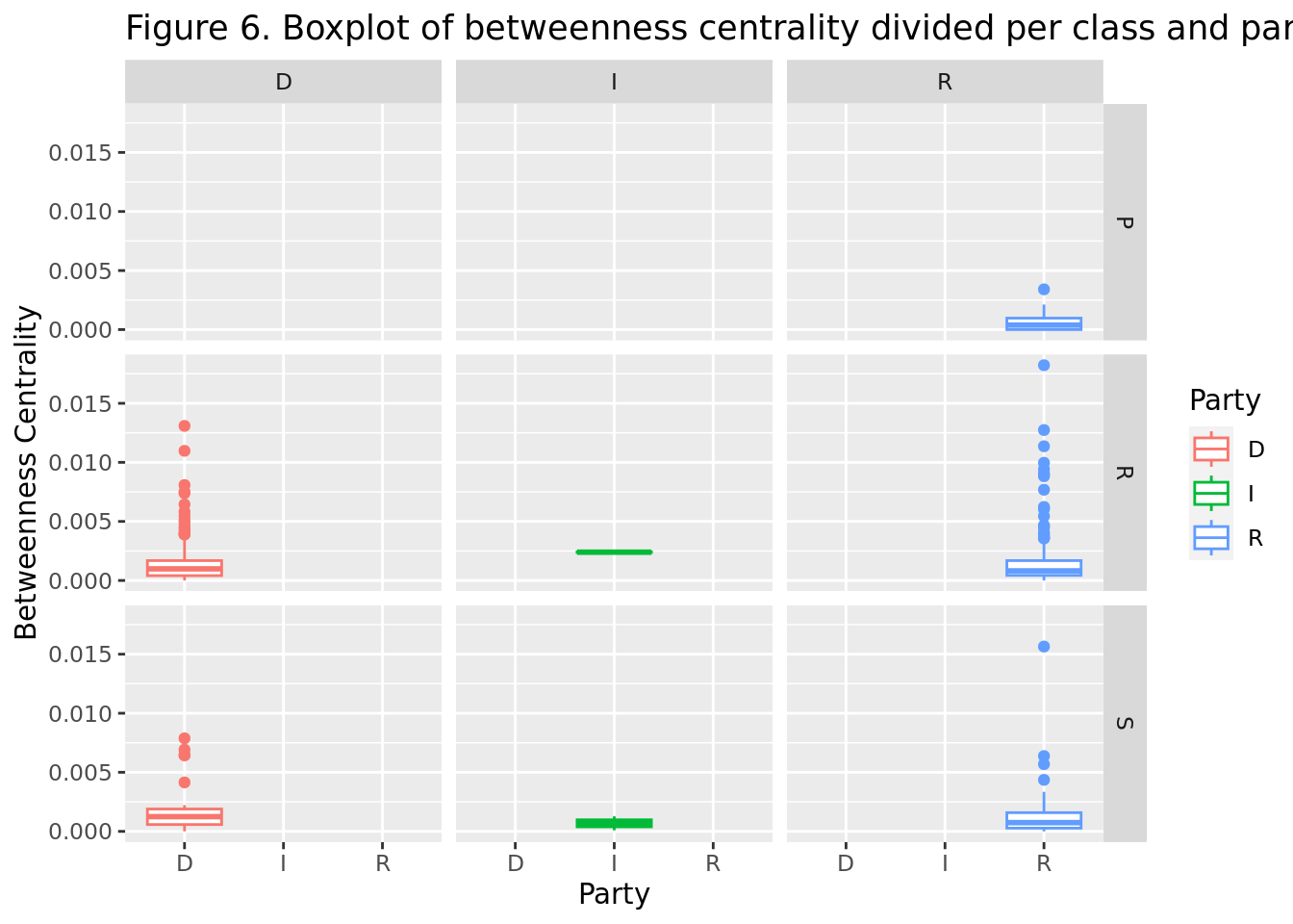
As we can see in Figure 6, the distribution of the betweenness centrality is very similar for all classes, however, both for the House of Representatives and the Senate, there are some outliers that score significantly higher than the rest of the data points. This can be explained by the fact that these individuals may be trend-setters, and occupy formal or informal leadership positions in their respective parties and political communities.
Let’s investigate the top 5 nodes with the highest betweenness centrality for each class and party.
| name | betweenness | state |
|---|---|---|
| joe courtney | 0.0130869 | connecticut |
| mary gay scanlon | 0.0109759 | pennsylvania |
| katie porter | 0.0080799 | california |
| dina titus | 0.0075046 | nevada |
| john larson | 0.0073901 | connecticut |
| name | betweenness | state |
|---|---|---|
| trent kelly | 0.0182250 | mississippi |
| mike johnson | 0.0127375 | louisiana |
| billy long | 0.0113627 | missouri |
| john curtis | 0.0099629 | utah |
| jim hagedorn | 0.0094138 | minnesota |
| name | betweenness | state |
|---|---|---|
| jack reed | 0.0078753 | rhode island |
| kirsten gillibrand | 0.0069148 | new york |
| doug jones | 0.0064576 | alabama |
| chris coons | 0.0064366 | delaware |
| chuck schumer | 0.0041431 | new york |
| name | betweenness | state |
|---|---|---|
| cindy hyde-smith | 0.0156456 | mississippi |
| tom cotton | 0.0063740 | arkansas |
| roger wicker | 0.0056867 | mississippi |
| marco rubio | 0.0043589 | florida |
| lisa murkowski | 0.0033480 | alaska |
| name | betweenness | state |
|---|---|---|
| gregorio kilili camacho sablan | 0.0024491 | northern mariana islands |
| justin amash | 0.0023432 | michigan |
| bernie sanders | 0.0012743 | vermont |
| angus king | 0.0000887 | maine |
4.3 Closeness centrality
The closeness centrality of a node is the inverse of the average length of the shortest paths from or towards all the other vertices in the graph. The more central a node is, the closer it is to all other nodes.
\[ C_{C}(i) = \frac{1}{\sum_{j \neq i} d_{ij}} \]
where \(d_{ij}\) is the shortest path between nodes \(i\) and \(j\).
In our case, I measured both the incoming and the outgoing closeness centrality
# Incoming closeness centrality
nodes$incloseness<-closeness(network, vids = V(network), mode = c("in"), normalized = FALSE)

# Outgoing closeness centrality
nodes$outcloseness<-closeness(network, vids = V(network), mode = c("out"), normalized = FALSE)
4.4 Eigenvector centrality
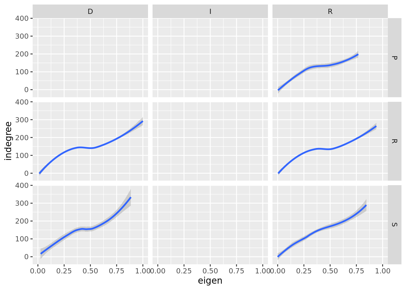
A natural extension of degree centrality is eigenvector centrality. While in-degree centrality awards one centrality point for every link a node receives, the eigenvector centrality of a node is proportional to the importance of its neighbours, whose importance is proportional to their neighbours, and so on so forth.
The ego function returns the vertices not farther than a given limit from another fixed vertex. Since it accepts vectors I am computing this measure for the potential of a node in being asource of information towards the other nodes. because of the different disposition of links within a network, some nodes will probably result in being more influential than others.
A node receiving many links does not necessarily have a high eigenvector centrality. It might just be that all the nodes it is connected to have low or null eigenvector centrality. Conversely, a node with high eigenvector centrality does not necessarily possess a large number of links because it might just be connected to a few individuals with high eigenvector centrality.
In the US Politician Network, the nodes with the highest eigenvector centrality are:
# Calculate eigenvector centrality
nodes$eigen<-eigen_centrality(network, directed = TRUE)$vector

ggplot(nodes, mapping=aes(x=eigen, y=indegree)) +
  geom_smooth() +
  facet_grid(class ~ party)
## `geom_smooth()` using method = 'loess' and formula = 'y ~ x'